Probabilistic bug hunting
Have you ever run into a bug that, no matter how careful you are trying to reproduce it, it only happens sometimes? And then, you think you've got it, and finally solved it - and tested a couple of times without any manifestation. How do you know that you have tested enough? Are you sure you were not "lucky" in your tests?
In this article we will see how to answer those questions and the math behind it without going into too much detail. This is a pragmatic guide.
The Bug
The following program is supposed to generate two random 8-bit integer and print them on stdout:
#include <stdio.h>
#include <fcntl.h>
#include <unistd.h>

/* Returns -1 if error, other number if ok. */
int get_random_chars(char *r1, char*r2)
{
	int f = open("/dev/urandom", O_RDONLY);

	if (f < 0)
		return -1;
	if (read(f, r1, sizeof(*r1)) < 0)
		return -1;
	if (read(f, r2, sizeof(*r2)) < 0)
		return -1;
	close(f);

	return *r1 & *r2;
}

int main(void)
{
	char r1;
	char r2;
	int ret;

	ret = get_random_chars(&r1, &r2);

	if (ret < 0)
		fprintf(stderr, "error");
	else
		printf("%d %d\n", r1, r2);

	return ret < 0;
}
On my architecture (Linux on IA-32) it has a bug that makes it print "error" instead of the numbers sometimes.
The Model
Every time we run the program, the bug can either show up or not. It has a non-deterministic behaviour that requires statistical analysis.
We will model a single program run as a Bernoulli trial, with success defined as "seeing the bug", as that is the event we are interested in. We have the following parameters when using this model:
- \(n\): the number of tests made;
- \(k\): the number of times the bug was observed in the \(n\) tests;
- \(p\): the unknown (and, most of the time, unknowable) probability of seeing the bug.
As a Bernoulli trial, the number of errors \(k\) of running the program \(n\) times follows a binomial distribution \(k \sim B(n,p)\). We will use this model to estimate \(p\) and to confirm the hypotheses that the bug no longer exists, after fixing the bug in whichever way we can.
By using this model we are implicitly assuming that all our tests are performed independently and identically. In order words: if the bug happens more ofter in one environment, we either test always in that environment or never; if the bug gets more and more frequent the longer the computer is running, we reset the computer after each trial. If we don't do that, we are effectively estimating the value of \(p\) with trials from different experiments, while in truth each experiment has its own \(p\). We will find a single value anyway, but it has no meaning and can lead us to wrong conclusions.
Physical analogy
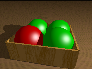
Another way of thinking about the model and the strategy is by creating a physical analogy with a box that has an unknown number of green and red balls:
- Bernoulli trial: taking a single ball out of the box and looking at its color - if it is red, we have observed the bug, otherwise we haven't. We then put the ball back in the box.
- \(n\): the total number of trials we have performed.
- \(k\): the total number of red balls seen.
- \(p\): the total number of red balls in the box divided by the total number of green balls in the box.
Some things become clearer when we think about this analogy:
- If we open the box and count the balls, we can know \(p\), in contrast with our original problem.
- Without opening the box, we can estimate \(p\) by repeating the trial. As \(n\) increases, our estimate for \(p\) improves. Mathematically: \[p = \lim_{n\to\infty}\frac{k}{n}\]
- Performing the trials in different conditions is like taking balls out of several different boxes. The results tell us nothing about any single box.
Estimating \(p\)
Before we try fixing anything, we have to know more about the bug, starting by the probability \(p\) of reproducing it. We can estimate this probability by dividing the number of times we see the bug \(k\) by the number of times we tested for it \(n\). Let's try that with our sample bug:
$ ./hasbug
67 -68
$ ./hasbug
79 -101
$ ./hasbug
error
We know from the source code that \(p=25%\), but let's pretend that we don't, as will be the case with practically every non-deterministic bug. We tested 3 times, so \(k=1, n=3 \Rightarrow p \sim 33%\), right? It would be better if we tested more, but how much more, and exactly what would be better?
\(p\) precision
Let's go back to our box analogy: imagine that there are 4 balls in the box, one red and three green. That means that \(p = 1/4\). What are the possible results when we test three times?
| Red balls | Green balls | \(p\) estimate |
|---|---|---|
| 0 | 3 | 0% |
| 1 | 2 | 33% |
| 2 | 1 | 66% |
| 3 | 0 | 100% |
The less we test, the smaller our precision is. Roughly, \(p\) precision will be at most \(1/n\) - in this case, 33%. That's the step of values we can find for \(p\), and the minimal value for it.
Testing more improves the precision of our estimate.
\(p\) likelihood
Let's now approach the problem from another angle: if \(p = 1/4\), what are the odds of seeing one error in four tests? Let's name the 4 balls as 0-red, 1-green, 2-green and 3-green:
The table above has all the possible results for getting 4 balls out of the box. That's \(4^4=256\) rows, generated by this python script. The same script counts the number of red balls in each row, and outputs the following table:
| k | rows | % |
|---|---|---|
| 4 | 1 | 0.39% |
| 3 | 12 | 4.69% |
| 2 | 54 | 21.09% |
| 1 | 108 | 42.19% |
| 0 | 81 | 31.64% |
That means that, for \(p=1/4\), we see 1 red ball and 3 green balls only 42% of the time when getting out 4 balls.
What if \(p = 1/3\) - one red ball and two green balls? We would get the following table:
| k | rows | % |
|---|---|---|
| 4 | 1 | 1.23% |
| 3 | 8 | 9.88% |
| 2 | 24 | 29.63% |
| 1 | 32 | 39.51% |
| 0 | 16 | 19.75% |
What about \(p = 1/2\)?
| k | rows | % |
|---|---|---|
| 4 | 1 | 6.25% |
| 3 | 4 | 25.00% |
| 2 | 6 | 37.50% |
| 1 | 4 | 25.00% |
| 0 | 1 | 6.25% |
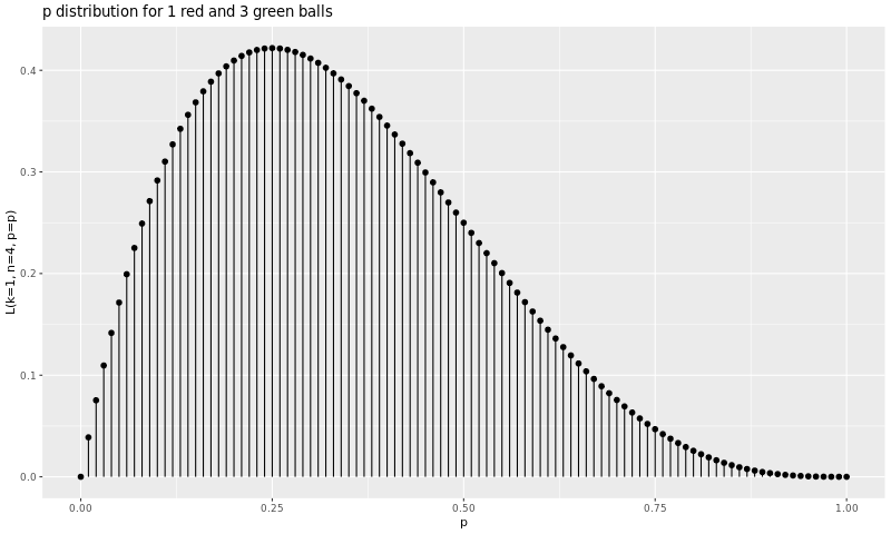
So, let's assume that you've seen the bug once in 4 trials. What is the value of \(p\)? You know that can happen 42% of the time if \(p=1/4\), but you also know it can happen 39% of the time if \(p=1/3\), and 25% of the time if \(p=1/2\). Which one is it?
The graph bellow shows the discrete likelihood for all \(p\) percentual values for getting 1 red and 3 green balls:
The fact is that, given the data, the estimate for \(p\) follows a beta distribution \(Beta(k+1, n-k+1) = Beta(2, 4)\) (1) The graph below shows the probability distribution density of \(p\):
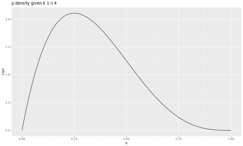
The R script used to generate the first plot is here, the one used for the second plot is here.
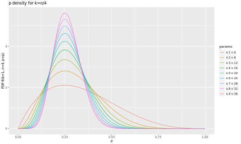
Increasing \(n\), narrowing down the interval
What happens when we test more? We obviously increase our precision, as it is at most \(1/n\), as we said before - there is no way to estimate that \(p=1/3\) when we only test twice. But there is also another effect: the distribution for \(p\) gets taller and narrower around the observed ratio \(k/n\):
Investigation framework
So, which value will we use for \(p\)?
- The smaller the value of \(p\), the more we have to test to reach a given confidence in the bug solution.
- We must, then, choose the probability of error that we want to tolerate, and take the smallest value of \(p\) that we can. A usual value for the probability of error is 5% (2.5% on each side).
- That means that we take the value of \(p\) that leaves 2.5% of the area of the density curve out on the left side. Let's call this value \(p_{min}\).
- That way, if the observed \(k/n\) remains somewhat constant, \(p_{min}\) will raise, converging to the "real" \(p\) value.
- As \(p_{min}\) raises, the amount of testing we have to do after fixing the bug decreases.
By using this framework we have direct, visual and tangible incentives to test more. We can objectively measure the potential contribution of each test.
In order to calculate \(p_{min}\) with the mentioned properties, we have to solve the following equation:
\[\sum_{k=0}^{k}{n\choose{k}}p_{min} ^k(1-p_{min})^{n-k}=\frac{\alpha}{2} \]
\(alpha\) here is twice the error we want to tolerate: 5% for an error of 2.5%.
That's not a trivial equation to solve for \(p_{min}\). Fortunately, that's the formula for the confidence interval of the binomial distribution, and there are a lot of sites that can calculate it:
- http://statpages.info/confint.html: \(\alpha\) here is 5%.
- http://www.danielsoper.com/statcalc3/calc.aspx?id=85: results for \(\alpha\) 1%, 5% and 10%.
- https://www.google.com.br/search?q=binomial+confidence+interval+calculator: google search.
Is the bug fixed?
So, you have tested a lot and calculated \(p_{min}\). The next step is fixing the bug.
After fixing the bug, you will want to test again, in order to confirm that the bug is fixed. How much testing is enough testing?
Let's say that \(t\) is the number of times we test the bug after it is fixed. Then, if our fix is not effective and the bug still presents itself with a probability greater than the \(p_{min}\) that we calculated, the probability of not seeing the bug after \(t\) tests is:
\[\alpha = (1-p_{min})^t \]
Here, \(\alpha\) is also the probability of making a type I error, while \(1 - \alpha\) is the statistical significance of our tests.
We now have two options:
- arbitrarily determining a standard statistical significance and testing enough times to assert it.
- test as much as we can and report the achieved statistical significance.
Both options are valid. The first one is not always feasible, as the cost of each trial can be high in time and/or other kind of resources.
The standard statistical significance in the industry is 5%, we recommend either that or less.
Formally, this is very similar to a statistical hypothesis testing.
Back to the Bug
Testing 20 times
This file has the results found after running our program 5000 times. We must never throw out data, but let's pretend that we have tested our program only 20 times. The observed \(k/n\) ration and the calculated \(p_{min}\) evolved as shown in the following graph:
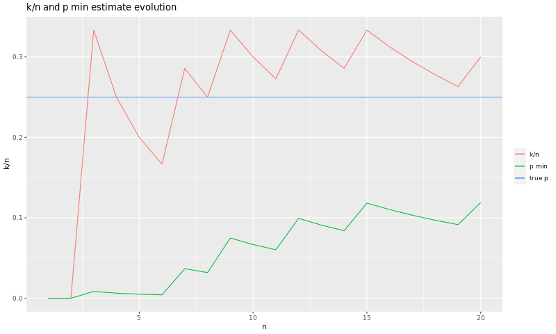
After those 20 tests, our \(p_{min}\) is about 12%.
Suppose that we fix the bug and test it again. The following graph shows the statistical significance corresponding to the number of tests we do:
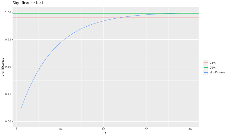
In words: we have to test 24 times after fixing the bug to reach 95% statistical significance, and 35 to reach 99%.
Now, what happens if we test more before fixing the bug?
Testing 5000 times
Let's now use all the results and assume that we tested 5000 times before fixing the bug. The graph bellow shows \(k/n\) and \(p_{min}\):
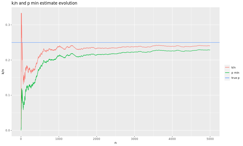
After those 5000 tests, our \(p_{min}\) is about 23% - much closer to the real \(p\).
The following graph shows the statistical significance corresponding to the number of tests we do after fixing the bug:
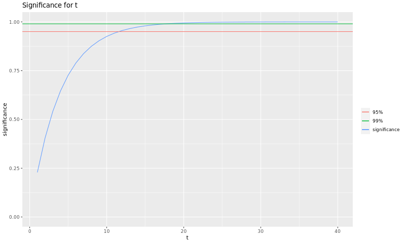
We can see in that graph that after about 11 tests we reach 95%, and after about 16 we get to 99%. As we have tested more before fixing the bug, we found a higher \(p_{min}\), and that allowed us to test less after fixing the bug.
Optimal testing
We have seen that we decrease \(t\) as we increase \(n\), as that can potentially increases our lower estimate for \(p\). Of course, that value can decrease as we test, but that means that we "got lucky" in the first trials and we are getting to know the bug better - the estimate is approaching the real value in a non-deterministic way, after all.
But, how much should we test before fixing the bug? Which value is an ideal value for \(n\)?
To define an optimal value for \(n\), we will minimize the sum \(n+t\). This objective gives us the benefit of minimizing the total amount of testing without compromising our guarantees. Minimizing the testing can be fundamental if each test costs significant time and/or resources.
The graph bellow shows us the evolution of the value of \(t\) and \(t+n\) using the data we generated for our bug:
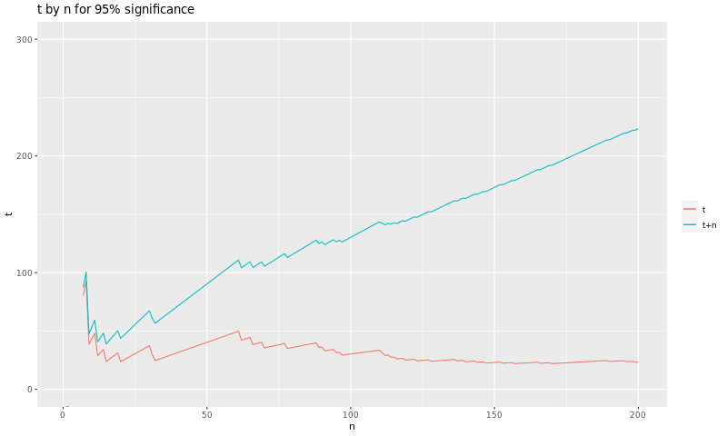
We can see clearly that there are some low values of \(n\) and \(t\) that give us the guarantees we need. Those values are \(n = 15\) and \(t = 24\), which gives us \(t+n = 39\).
While you can use this technique to minimize the total number of tests performed (even more so when testing is expensive), testing more is always a good thing, as it always improves our guarantee, be it in \(n\) by providing us with a better \(p\) or in \(t\) by increasing the statistical significance of the conclusion that the bug is fixed. So, before fixing the bug, test until you see the bug at least once, and then at least the amount specified by this technique - but also test more if you can, there is no upper bound, specially after fixing the bug. You can then report a higher confidence in the solution.
Conclusions
When a programmer finds a bug that behaves in a non-deterministic way, he knows he should test enough to know more about the bug, and then even more after fixing it. In this article we have presented a framework that provides criteria to define numerically how much testing is "enough" and "even more." The same technique also provides a method to objectively measure the guarantee that the amount of testing performed provides, when it is not possible to test "enough."
We have also provided a real example (even though the bug itself is artificial) where the framework is applied.
As usual, the source code of this page (R scripts, etc) can be found and downloaded in https://github.com/lpenz/lpenz.github.io
